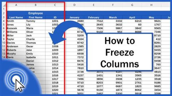
To freeze multiple rows (starting with row 1), select the row below the last row you want frozen and click Freeze Panes. To freeze multiple columns, select the column to the right of the last column you want frozen and click Freeze Panes. Say you want to freeze the top four rows and leftmost three columns.

.

Hereof, how do I freeze columns in Excel for Mac?

To freeze the first row and column, open your Excel spreadsheet. Select cell B2. Then select the Layout tab from the toolbar at the top of the screen. Click on the Freeze Panes button and click on the Freeze Panes option in the popup menu.

Likewise, how do you select a whole column in Excel on a Mac? Simply highlight any cell within the row or column you'd like to work with. To select an entire column: Ctrl + Spacebar. To select an entire row: Shift + Spacebar.

Furthermore, how do I freeze two columns in Excel 2019?

Freezing Columns and Rows

1. To freeze a set of columns and rows at the same time, click on the cell below and to the right of the panes you want to freeze.
2. With the proper cell selected, select the “View” tab at the top and click on the “Freeze Panes” button, and select the “Freeze Panes” option in the drop-down.

How do I freeze multiple columns in Excel 2016?

How to Freeze Rows and Columns in Excel 2016

1. Select the row right below the row or rows you want to freeze. If you want to freeze columns, select the cell immediately to the right of the column you want to freeze. In this example, we want to freeze rows 1 to 6, so we've selected row 7.
2. Go to the View tab.
3. Select the Freeze Panes command and choose "Freeze Panes."

Related Question Answers

How do I make the first row in Excel a header?

Go to the "Insert" tab on the Excel toolbar, and then click the “Header & Footer” button in the Text group to start the process of adding a header. Excel changes the document view to a Page Layout view. Click on the top of your document where it says “Click to Add Header,” and then type the header for your document.

Why is Excel freezing the wrong panes?

When you no longer need the rows or columns locked in place, you in turn can unfreeze them. To unlock the rows or columns, navigate to the View tab, choose Freeze Panes, and then Unfreeze Panes. It's a little simpler in Excel 2003: choose Window, and then Freeze Panes or Window, and then Unfreeze Panes, respectively.

How do I make a floating header in Excel?

Here is how you do it:

1. This moment is the key - select the cell just below the rows you want to freeze, and to the right of such columns if needed.
2. Open the View tab in Excel and find the Freeze Panes option in the Window group.
3. Click on the little arrow next to it to see all the options, and choose to Freeze Panes.

How do I freeze columns in Excel 2010?

To freeze rows:

1. Select the row below the rows you want frozen. For example, if you want rows 1 and 2 to always appear at the top of the worksheet even as you scroll, then select row 3.
2. Click the View tab.
3. Click the Freeze Panes command.
4. Select Freeze Panes.
5. A black line appears below the rows that are frozen in place.

Where is freeze panes in Excel?

Freeze columns and rows

1. Select the cell below the rows and to the right of the columns you want to keep visible when you scroll.
2. Select View > Freeze Panes > Freeze Panes.

How do I freeze rows and columns at the same time in Excel 2010?

To freeze the first row and column, open your Excel spreadsheet. Select cell B2. Then select the View tab from the toolbar at the top of the screen and click on the Freeze Panes button in the Window group. Then click on the Freeze Panes option in the popup menu.

How do you freeze rows in sheets?

To pin data in the same place and see it when you scroll, you can freeze rows or columns.

1. On your computer, open a spreadsheet in Google Sheets.
2. Select a row or column you want to freeze or unfreeze.
3. At the top, click View. Freeze.
4. Select how many rows or columns to freeze.

How do I freeze rows and columns at the same time?

You can also freeze both columns and rows at the same time. To freeze both rows and columns, select the upper left cell in the data you don't want to freeze. Then choose Freeze Panes from the menu. Now the rows above this cell, and the columns to the left of this cell will be frozen, and remain visible as you scroll.

How do I freeze multiple rows and columns in Excel at the same time?

To lock more than one row or column, or to lock both rows and columns at the same time, choose the View tab, and then click Freeze Panes. You will want your cursor to be below the row(s) you want to freeze and to the right of any column(s) you want to freeze.

What is the shortcut key to freeze a column in Excel?

Freeze panes: Put the active cell in the desired location, and press Alt+w and then F. To remove the freeze panes, use the same shortcut.

What is the shortcut to lock cells in Excel for Mac?

It's much faster and easier than typing $ characters manually. To convert an existing formula, enter cell edit mode, place the cursor in or next to the reference you'd like to convert, then use the shortcut. Note: in Excel 2016 for the Mac, you can also use fn + F4.

How do I freeze rows and columns at the same time in Excel 2003?

To freeze the first row and column, open your Excel spreadsheet. Select cell B2. Then under the Window menu, select Freeze Panes. Now when you scroll, you should still continue to see row 1 and column A.

Why is freeze panes GREY?

To enable the Freeze Panes command again, you must choose either the Normal or Page Break Preview commands. You'll have to manually restore any frozen panes that you lost when you chose Page Layout view. Figure 1: Excel's Page Layout command disables the Freeze Panes command and unfreezes rows/columns, as well.

How do I freeze rows and columns at the same time in Excel 2007?

To freeze the first row and column, open your Excel spreadsheet. Select cell B2. Then select the View tab from the toolbar at the top of the screen and click on the Freeze Panes button in the Window group. Then click on the Freeze Panes option in the popup menu.

How do you keep a cell fixed in Excel?

Keep formula cell reference constant with the F4 key 1. Select the cell with the formula you want to make it constant. 2. In the Formula Bar, put the cursor in the cell which you want to make it constant, then press the F4 key.

How do you merge cells on Excel?

To merge a group of cells:

1. Highlight or select a range of cells.
2. Right-click on the highlighted cells and select Format Cells.
3. Click the Alignment tab and place a checkmark in the checkbox labeled Merge cells.

Where is freeze panes in Excel Mac?

To freeze the first row and column, open your Excel spreadsheet. Select cell B2. Then select the Layout tab from the toolbar at the top of the screen. Click on the Freeze Panes button and click on the Freeze Panes option in the popup menu.

How do I freeze cells in Excel 365?

Freeze columns and rows to keep them in view while you scroll through your data.

1. Select the cell below the rows, and to the right of the columns you want to freeze.
2. Click View > Freeze Panes > Freeze Panes.

How do you group tabs in Excel?

Press and hold down the Ctrl key, and click the worksheet tabs you want to group. Tip: If you want to group consecutive worksheets, click the first worksheet tab in the range, press and hold the Shift key, and click the last worksheet tab in the range.